The exoplanet catalogue1 of 3
A catalogue of alien worlds
A procedural-visualisation interface to the Open Exoplanet Catalogue
System descriptionJuly 202629 min read
First published at exoplanet-catalogue.vercel.app.
Abstract
More than four thousand planetary systems beyond the Sun have been confirmed, yet we know each exoplanet through a small set of numbers: period, radius or minimum mass, orbital distance, and a few properties of its star. The public usually meets that record as either a table or an artist's impression, with little indication of how the picture relates to the measurements.
I took a third route. This interface renders all 4,081 systems in the Open Exoplanet Catalogue as explorable 3D scenes. A documented classifier and procedural shader derive each planet's appearance from its recorded physical parameters. The site has a curated catalogue, an orbital viewer with Keplerian propagation and a galactic map that positions every system by right ascension, declination and distance. At build time, one pipeline turns the catalogue XML into JSON and another uses the live shaders to bake the thumbnails.
The awkward engineering problem is scale. A scene may contain a star, planets a hundredth of its size and orbits reaching seventy-nine thousand scene units, all inside 32-bit GPU arithmetic. The viewer uses relative-to-eye orbit rendering and split-precision camera arithmetic to hold it together. Star colour comes from effective temperature as blackbody colour, while the map places systems from their archival astrometry at one parsec per scene unit. The companion pieces cover planet rendering and the wider history of exoplanet visualisation. I have not yet run a user study; the evaluation section sets out what one should test.
1. Introduction
The first planet found orbiting a Sun-like star was announced in 1995 (Mayor & Queloz 1995). Three decades later the confirmed count is in the thousands and grows weekly. Exoplanets are objects of intense public fascination that remain almost entirely invisible. Nearly every known exoplanet was detected indirectly, as a periodic dimming of its star's light or a periodic wobble in its star's spectrum, and even the few dozen imaged directly appear as unresolved points of light (Marois et al. 2008). There is no photograph of an exoplanet's surface, and there will be none for the foreseeable future.
What exists instead is a catalogue: for each system, a set of measured and inferred quantities, with uncertainties, maintained in public databases (Akeson et al. 2013; Schneider et al. 2011; Rein 2012). The catalogue is open, machine-readable, and hard to see. A table of periods and radii does not communicate that TRAPPIST-1's seven worlds huddle closer to their star than Mercury does to the Sun, or that a hot Jupiter's year lasts four days, or what it means for a planet to be tidally locked. I wanted to make that data legible as a set of places without disguising how little we know about their appearance.
The site renders the entire Open Exoplanet Catalogue, 4,081 system records vendored as XML and synchronised weekly with the upstream repository, as an interactive site: a catalogue page of featured systems, a three-dimensional viewer for any system, and a star map of the whole catalogue. The main design rule, developed at length in the companion paper Plausible Worlds from Sparse Parameters, is that a planet's rendered appearance is a deterministic function of its recorded parameters: a classification pipeline assigns each planet one of sixteen physically motivated types, and a procedural shader renders that type. Nothing is hand-painted, and nothing is random between visits.
What the work adds
React, WebGL scene graphs and procedural noise shaders are all established practice. The useful work is in applying them to the whole catalogue and recording what that required.
- Parameter-derived rendering covers every system in the catalogue, including the sparse majority for which only two or three parameters are recorded, with documented fallbacks for every missing quantity. The derivation extends beyond the planets: star colour is computed from temperature, and system positions from archival astrometry.
- Precision rendering lets the viewer hold bodies from 0.08 to thousands of scene units across orbits up to ~10⁵ units in 32-bit GPU arithmetic, using relative-to-eye orbit rendering with high/low float splitting, periapsis clearance for close-in planets, and unit disambiguation for binary separations.
- The bake pipeline uses the live GLSL shaders to pre-render the catalogue's thumbnails through a headless browser, so the still and interactive views cannot drift apart.
- The star map parses right ascension, declination and distance at build time into a Cartesian index, then draws a single point cloud at true parsec scale. The zodiac constellations projected through the same transform for orientation.
2. Background: what the catalogue contains
2.1 The Open Exoplanet Catalogue
The Open Exoplanet Catalogue (OEC) is a community-maintained, decentralised
database of exoplanet discoveries, stored as one XML file per system under
version control (Rein 2012). It was chosen over the institutional alternatives
(the NASA Exoplanet Archive, exoplanet.eu) for two properties that suit a
self-contained web application: the entire catalogue is a directory of files
that can be vendored into the repository, and its hierarchical schema
represents multiple-star systems natively. A <binary> element contains
stars, planets, or further binaries, so a hierarchical triple like 16 Cygni,
two stars in a close pair with a third carrying the planet, is a tree, not a
footnote.
The trade-off is currency. Community maintenance has slowed relative to the institutional archives, and the vendored copy's 4,081 system files should be read as the OEC's coverage, not the field's: the NASA Exoplanet Archive's confirmed-planet count is substantially higher. The repository syncs with upstream weekly (a scheduled job, Mondays 06:00 UTC), so the gap is upstream, not local. The figures the site shows are the catalogue's.
2.2 The anatomy of a system record
A system record contains, at most: a name and aliases; right ascension, declination, and distance (parsecs, with error bounds); for each star, mass, radius, effective temperature, spectral type, metallicity, magnitudes, and age; for each planet, mass (sometimes only m sin i), radius, period, semi-major axis, eccentricity, inclination, periastron, discovery method and year, and a prose description. Binary systems add separations (in arcseconds and/or AU) and position angles.
The operative phrase is at most. The catalogue's sparsity is structural, not incidental: transit surveys yield radii but often no mass; radial-velocity detections yield minimum masses but no radius; many entries record little more than a period and a host star. Every downstream stage of the system, classification, scaling, orbit propagation, therefore begins from the premise that any field may be absent, and the fallback chain for each quantity is part of the design (Section 3.5, and the companion paper §3).
3. The system
3.1 Design principles
Five tenets served as tiebreakers throughout.
- Derive, don't decorate. A planet's look must be a function of its data. The same record renders the same world on every visit (appearance is seeded deterministically); a different record renders a different world. The same rule covers the stars (colour from temperature, §3.5) and the map (position from astrometry, §3.6).
- Legibility over literal scale. Bodies are enlarged relative to their orbits, close orbits are kept clear of the star's surface, and time is compressed, while the relative quantities within a system, orbital rates, size orderings, positions on the sky, are preserved.
- The catalogue is the interface. Browse views, featured cards, and the star map all resolve to the same underlying records; there is no separate "content" layer that could drift from the data.
- Live and baked must agree. Pre-rendered imagery is produced by the same shaders as the interactive scene, through the bake pipeline, so a thumbnail is a genuine still of the world the viewer will show.
- Dark, editorial, quiet. The visual register is a black-background editorial catalogue, closer to a printed atlas than to an application, so that the procedural worlds, not the chrome, carry the interest.
3.2 Architecture and stack
The application is a server-rendered React Router site with a three.js scene graph mounted per route.
| Layer | Component |
|---|---|
| Framework | React Router 7.13 (framework mode, SSR on, file-system routes) |
| 3D | three.js 0.172 via @react-three/fiber 8.17, drei 9.120 |
| Shaders | Hand-written GLSL (planet ~2,100 lines; star; nebula; orbit lines) |
| Colour | chroma-js blackbody temperature scale for all stellar colour |
| Data | Vendored OEC XML → build-time JSON (xml2js 0.6) |
| Post-processing | @react-three/postprocessing (SMAA, ACES tone mapping et al.) |
| Bake | Playwright headless Chromium, 512 px PNG per featured system |
| Hosting | Vercel (git-connected build); Node ≥ 18 |
Three routes carry the experience: the catalogue index (/), the system
viewer (/system/:filename), and the star map (/galaxy). A fourth route
(/planet-bake) exists only as the bake pipeline's render target.
3.3 The data pipeline
A prebuild script (scripts/prebuild-data.js) runs before every build and
converts the 4,081 XML files once, so that no XML is parsed at request time.
- Per-system JSON. Each system file is parsed (xml2js, attributes
discarded) and written to
data-json/<name>.json. The system viewer's loader reads this JSON from disk (or, client-side, over HTTP); a missing file is a 404, not a crash. - The galaxy index. For every system with usable coordinates, the script extracts right ascension, declination and distance, converts them to radians and parsecs, and projects to Cartesian coordinates (§3.6). Each index record carries name, filename, position, distance, and planet count. Systems without coordinates are skipped and counted; the script reports parsed, skipped and indexed totals on every run.
The generated data-json/ directory is gitignored and rebuilt per checkout;
the vendored XML is the only checked-in data artefact.
3.4 The catalogue surface
The index page presents a masthead, a stats strip, and a grid of systems.
Twenty-one systems are editorially selected (catalogueSystems.ts):
TRAPPIST-1, Proxima Centauri, 51 Pegasi, Kepler-442, HR 8799, 55 Cancri, the
Solar System as reference, and others, each with a blurb, a featured planet,
tags drawn from a fixed eight-tag vocabulary (habitable zone, rocky, gas
giant, historic, nearest, exotic, multi-planet), and a seed. The cards are
curated pointers: each links into the same system-viewer route as any search
result, so curation adds narrative without forking the data path. Card
imagery comes from the bake pipeline (§3.7).
The masthead behind the title is not an image but a live shader planet at 1300 × 1300 render resolution, cycling through nine representative types on a six-second interval, draggable with inertia. It is the first statement of the project's thesis: the artwork is the data pipeline running.
3.5 The system viewer
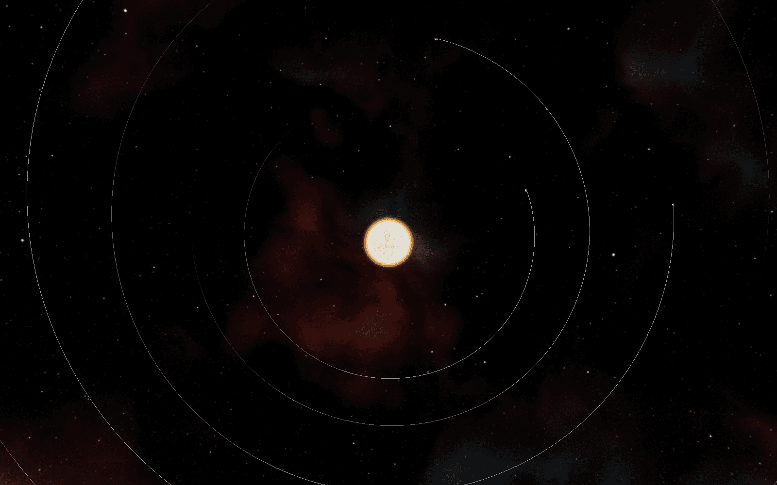
The viewer renders one system as a navigable scene: star (or star hierarchy), planets on animated orbits, habitable-zone annulus, orbit lines, nebula and Milky Way skybox, under cinematic post-processing.
Scale model
One astronomical unit maps to 2,000 scene units; one solar
radius is then 9.30 units and one Jupiter radius 0.926 (the physical ratios,
1 AU = 215.032 R☉ and 1 R☉ = 10.045 R_Jup, are kept in code as named
constants). Bodies are additionally scaled by a user-adjustable bodyScale
(default ×3), since at true scale a planet at catalogue distances is
subpixel; orbits keep their true relative proportions.
Keplerian propagation
Each planet's position is computed per frame from first principles: mean anomaly advances as (elapsed/period) scaled by a global time-compression factor, plus a phase offset (the recorded periastron where present, else a deterministic name-hash so that co-orbital planets do not stack); Kepler's equation M = E − e sin E is solved by Newton–Raphson (at most 30 iterations, tolerance 10⁻⁸, seeded at E = π for e > 0.8, following standard practice; Danby 1988, Colwell 1993); true anomaly and radius follow, and near-circular orbits (e < 10⁻⁶) short-circuit to the trigonometric case. Because every planet advances by elapsed/period, relative orbital rates within a system are correct even though absolute time is compressed.
Periapsis clearance
Because bodies are scaled and orbits are not, a close-in planet's rendered orbit can fall inside its star's rendered surface (WASP-12 b, at 0.023 AU around a swollen star, is the canonical case, and rendered literally it reads as an error rather than as the genuinely remarkable fact that hot Jupiters skim their stars). The viewer therefore enforces clearance: if periapsis a(1 − e) falls below the star's scene radius plus 1.6× the planet's, the semi-major axis is pushed out to clear it, and the catalogue values continue to drive everything else.
Stars from temperature
A star's whole appearance derives from two catalogue numbers, effective temperature and radius. Colour is blackbody colour, computed with chroma-js's temperature scale rather than assigned by spectral class: the point light that illuminates the system takes the blackbody value directly, and the surface shader's tint is derived from the ratio of the blue to red channels of that same blackbody colour, clamped to a working range, so that M dwarfs render deep orange, the Sun sits near the middle of the scale, and O stars run blue-white, continuously rather than in class steps. The corona and flare sprites reuse the same scale at reduced temperatures (rays at 0.85×, flares at 0.75×), so the star's fringe reads cooler than its disc. The surface itself is three rotating layers of four-dimensional simplex noise at five octaves, animated in time for granulation. Where the catalogue records only a spectral type, a lookup supplies the temperature (M 3,000 K through O 40,000 K), and the recorded visual magnitude sets the scene light's intensity within a clamped range.
Binaries
The OEC's hierarchical <binary> trees are rendered
recursively: each binary node splits into two children (stars, planets, or
nested binaries) placed on opposite sides of the barycentre with mass-weighted
offsets and the recorded position angle. One data hazard is disambiguated
explicitly. The catalogue may record separation twice, in arcseconds and in
AU, and naive parsing takes the arcsecond value first, an error of three
orders of magnitude; the loader takes the maximum of the numeric candidates,
on the grounds that the AU figure is always the larger. Separations are
further clamped to a maximum scene offset, because float32 matrix arithmetic
degrades visibly beyond ~10⁶ units.
Orbit lines at distance: relative-to-eye rendering
The most instructive
numerical problem was the outermost orbits. At Pluto-scale distances (~79,000
scene units) a float32 vertex position has a granularity of roughly 0.005
units, and the standard modelView transform subtracts two nearly equal large
numbers (vertex − camera), so orbit lines visibly jittered and breathed as the
camera moved. The fix is the relative-to-eye technique from virtual-globe
rendering (Cozzi & Ring 2011): each orbit vertex is split at build time into a
high part (the float32-rounded value, via Math.fround) and a low part (the
residual), stored as two attributes; the camera position, transformed into the
orbit's local frame each frame, is split the same way; and the vertex shader
computes (pos_high − cam_high) + (pos_low − cam_low), in which the large high
parts cancel exactly and the residuals carry the precision. The modelView's
translation component is discarded (only its rotation is applied), so no large
translation ever enters the GPU pipeline. Orbit lines additionally fade out as
the camera approaches a planet, ramping over 5–20 % of the semi-major axis, so
that the line never slices through a close-up view. Segment counts adapt to
circumference (256–8,192).
Controls and locks
Camera control (drei CameraControls) enforces a
minimum approach distance of 1.15× a selected body's rendered radius, so that
one cannot dolly inside a star, and a follow mode re-targets the camera each
frame without damping, because damped following visibly lags a fast
hot-Jupiter. Tidally locked planets (as flagged by the classification) do not
rotate; their cloud layers are slaved to surface rotation at 1.15×
(super-rotation), so that clouds on a locked world correctly stand still with
it rather than counter-rotating.
The habitable zone, per star
The annulus is derived in two steps from the stellar record. Luminosity comes from Stefan–Boltzmann, L/L☉ = (R/R☉)²·(T/5778 K)⁴, when temperature and radius are recorded, and from a mass–luminosity power law otherwise, with the exponent chosen by spectral type (≈5.5 for M dwarfs falling to ≈3.5 for the hottest classes). The zone's edges then follow from the effective-flux formulation of Kopparapu et al. (2013): the runaway-greenhouse and maximum-greenhouse boundaries are quartic polynomials in the star's temperature offset from the Sun's, and each boundary distance is D = √(L/S_eff) AU. The polynomials are the interesting part. A naive habitable zone just rescales the Sun's by luminosity; Kopparapu's flux thresholds themselves move with stellar temperature, because a planet responds to the spectrum and not only the wattage: redder light is absorbed more efficiently by water vapour and reflected less by ice, so the zone around an M dwarf sits at measurably lower flux than the Sun's. Around TRAPPIST-1 the entire zone lies within a twentieth of an astronomical unit.
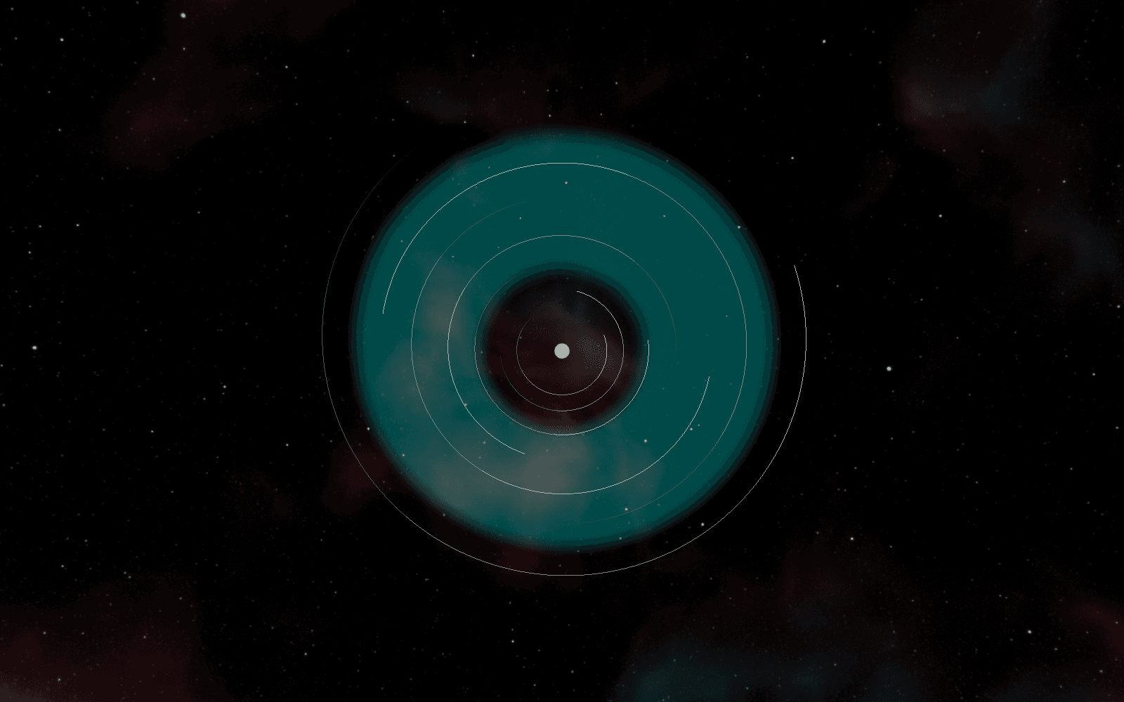
The same derivation serves two consumers: this annulus, and the classification pipeline's positioning of temperate worlds within the zone (companion paper, §2.3), so the ring the viewer draws and the palette a temperate planet receives cannot disagree. The render is an additive, double-sided, soft-edged ring, its geometry padded 30 % beyond the computed bounds for the fade, tilted to the mean inclination of the system's planets, off by default and toggled from the toolbar.
3.6 The star map
The /galaxy route is the catalogue drawn as a place: every indexed system
positioned where it actually is, at one parsec per scene unit, with Sol at the
origin.
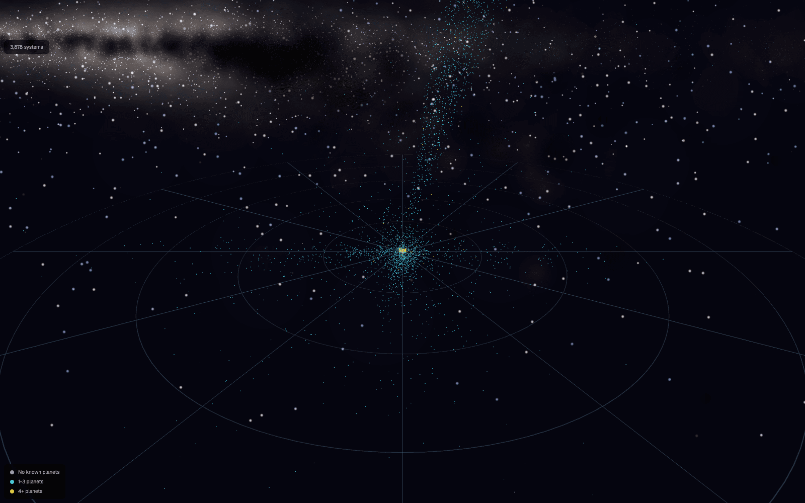
The positions are computed at build time from the catalogue's own archival astrometry. Right ascension is recorded in hours, minutes and seconds and converts at fifteen degrees per hour; declination in signed degrees, minutes and seconds; both reduce to radians and, with the distance in parsecs, project to Cartesian coordinates: x = d·cos δ·cos α, y = d·cos δ·sin α, z = d·sin δ. Systems missing any of the three values are skipped and counted, and each surviving record carries name, filename, position, distance and planet count into a single galaxy index that the route loads whole.
Rendering four thousand systems is then one draw call. Positions and colours
are packed into two Float32Arrays and drawn as a single THREE.Points cloud,
with the catalogue's z-up remapped to the renderer's y-up. At one parsec
per unit the whole known exoplanet population sits within a few thousand
units of the origin, comfortably inside float32, so the map needs none of the
split-precision machinery of §3.5. An equatorial reference grid draws
concentric rings at 200 to 1,000 parsecs with radial spokes every 30°, and the
twelve zodiac constellations are projected through the same transform, the
familiar two-dimensional sky embedded in the true three-dimensional
distribution, which is what gives a newcomer their bearings. Hover and
selection surface each system's name, distance and planet count, and
click-through opens the system viewer: the map and the viewer are two
projections of the same records.
Drawn this way, properties of the real population become legible that no table conveys: the Kepler field prints as a dense cone on one side of the sky, the survey's fixed stare made visible, and the population thins with distance because detection does, not because planets do, the geometric bias the companion survey paper discusses.
3.7 The bake pipeline
Thumbnails are not exported art; they are captured output. A Node script
launches headless Chromium (Playwright), starts the site on a local port,
navigates to the dedicated /planet-bake route for each of the 21 curated
slugs, which classifies the featured planet from its real catalogue record and
renders it with the production shaders, and screenshots a 512-pixel PNG per
system into public/planet-thumbs/. Because bake and live share one shader
and one classification, a change to either regenerates both looks with a
single command. (The pipeline exists because the live shader at full quality
is too costly to run two dozen times on a catalogue page; the masthead runs
exactly one live instance.)
4. Related work
Interactive astronomy visualisation
NASA's Eyes on Exoplanets renders the known exoplanet population as navigable 3D, from institutionally curated data; OpenSpace (Bock et al. 2020) and Gaia Sky (Sagristà et al. 2019) target planetarium-grade contextualisation of astronomical catalogues, with the Gaia star catalogue as the paradigm case; Celestia and Stellarium are the long-standing open-source ancestors. This project differs in two commitments: the appearance layer is parameter-derived per planet, rather than a stock texture per class, and the whole pipeline, data, classification, shaders and bake, is a single small open codebase intended to be read. The comparative field is the subject of the third companion paper.
Procedural planets
Procedural planetary surfaces have a deep graphics lineage (Perlin 1985; Musgrave et al. 1989; Ebert et al. 2003) and a contemporary commercial one (Space Engine; No Man's Sky). The distinction here is the grounding: procedural technique is subordinated to a documented classification of real catalogue records. That layer is the subject of the companion paper, which carries the related work on noise and shading.
Precision rendering at planetary scale
The high/low float splitting used for orbit lines is standard in virtual-globe engines (Cozzi & Ring 2011), where Earth-sized coordinates exceed float32; the contribution here is its application to orbit polylines in a catalogue viewer, together with clamped binary offsets at extreme separations. A full floating-origin refactor is on the roadmap.
Data infrastructure
The OEC's design rationale is given by Rein (2012); the institutional archives by Akeson et al. (2013) and Schneider et al. (2011). The prebuild-to-JSON pattern follows ordinary static-site practice and claims no novelty.
5. Evaluation
No empirical results are reported; this section specifies the evaluation the system is designed to support.
Performance
Frame-time distributions (median, p95) across a stratified sample of systems: single-star single-planet, high-multiplicity (TRAPPIST-1, Kepler-90), hierarchical binaries (16 Cygni), and extreme-scale orbits, on reference hardware tiers, with and without post-processing; together with time-to-first-frame for the viewer route and bake-pipeline wall time.
Numerical fidelity
Orbit-line stability quantified as screen-space vertex displacement across camera dollies at fixed logical positions, RTE on against RTE off; propagation accuracy against a reference double-precision ephemeris over 10³ orbits (drift in phase); and an exhaustive count of the catalogue cases where clearance rules (periapsis, binary separation) adjust rendered geometry.
Classification audit
Since the appearance layer's validity rests on the classification, a sample of catalogue planets with published characterisation (confirmed hot Jupiters, the TRAPPIST-1 planets, known super-puffs) should be checked against assigned types by a domain reviewer, with disagreement rates reported per branch of the decision tree. This audit is specified in detail in the companion paper.
Readers
A task-based study with non-specialist readers, locate a system, state which of two planets is hotter and why, judge whether an orbit's speed difference is meaningful, against the same tasks on a tabular interface, measuring accuracy and self-reported understanding, with explicit probes for the misconception risks the companion papers identify as the main hazard of the genre: do participants believe they saw photographs? do they report the continents as known?
6. Limitations
Stats derivation
The stats strip's headline figure labelled "confirmed" is the live system-file count (4,081), while the "systems" (4,231), habitable-zone (62) and earth-like (147) figures are literals; deriving all four from the index at build time is scheduled work.
Orbital orientation is partial
Only inclination is applied to an orbit's plane, as a single tilt of π/90 per recorded degree (twice the physical angle); longitude of the ascending node and argument of periapsis are not represented in 3D, and periapsis enters only as a phase offset. Rendered orbital orientation is illustrative rather than to scale.
The viewer is an interpretive diagram, not a simulation
Bodies ×3 (adjustable), orbits at true relative proportion, periapses cleared of the stellar surface, binary separations capped at 20,000 units, time compressed by a global factor. Within-system comparisons (rates, orderings, ratios) are preserved; absolute measurements are not recoverable from the screen.
One catalogue, ageing
Coverage and currency are bounded by the OEC. Systems confirmed since the community catalogue's maintenance slowed are absent, and no cross-check against the NASA archive is performed. Weekly sync guarantees freshness against upstream only.
Sparse-data planets render with equal confidence
A planet known only by period and m sin i renders as vividly as TRAPPIST-1 e. The classification pipeline's fallback chain (companion paper §3) covers the derivation, but the interface does not yet surface per-planet data completeness; a "what is this picture based on?" affordance remains roadmap.
No moons; controversial entries included
Satellites in the catalogue are
not rendered. Planets flagged Controversial upstream are rendered without a
visual distinction.
No user study has been run
All claims about legibility are design rationale, not measured outcomes (Section 5).
7. Conclusion
The result turns a public exoplanet catalogue into explorable scenes. Vendored XML feeds a classification-driven appearance layer, a Keplerian viewer built to cope with float32 at catalogue scale, temperature-derived star colours and a map based on the archive's own astrometry. The approach is useful beyond astronomy: derive visible properties from the record wherever possible, and keep that record close enough to inspect.
The interface still cannot tell a reader how much of each planet is known. Plausible Worlds from Sparse Parameters deals with the line between measurement and plausible fiction. From Data Point to Destination asks what this kind of interface can do for public understanding. Those are harder questions than rendering four thousand planets, which is faintly annoying.
Acknowledgements
This project exists because the Open Exoplanet Catalogue's maintainers chose openness and decentralisation (Rein 2012), and because the three.js, react-three-fiber and wider WebGL communities made planetary-scale rendering in the browser a practical undertaking. The Milky Way skybox derives from NASA imagery. The classification stands on the exoplanet characterisation literature cited in the companion paper.
References
Exoplanet data infrastructure
- Rein, H. (2012). A proposal for community driven and decentralized astronomical databases and the Open Exoplanet Catalogue. arXiv:1211.7121.
- Akeson, R. L., et al. (2013). The NASA Exoplanet Archive: Data and Tools for Exoplanet Research. PASP 125, 989.
- Schneider, J., Dedieu, C., Le Sidaner, P., Savalle, R., & Zolotukhin, I. (2011). Defining and cataloging exoplanets: the exoplanet.eu database. A&A 532, A79.
Discoveries and characterisation
- Mayor, M., & Queloz, D. (1995). A Jupiter-mass companion to a solar-type star. Nature 378, 355–359.
- Marois, C., et al. (2008). Direct Imaging of Multiple Planets Orbiting the Star HR 8799. Science 322, 1348–1352.
- Gillon, M., et al. (2017). Seven temperate terrestrial planets around the nearby ultracool dwarf star TRAPPIST-1. Nature 542, 456–460.
- Kopparapu, R. K., et al. (2013). Habitable Zones around Main-sequence Stars: New Estimates. ApJ 765, 131.
Orbital mechanics and numerics
- Danby, J. M. A. (1988). Fundamentals of Celestial Mechanics, 2nd ed. Willmann-Bell.
- Colwell, P. (1993). Solving Kepler's Equation Over Three Centuries. Willmann-Bell.
- Cozzi, P., & Ring, K. (2011). 3D Engine Design for Virtual Globes. CRC Press. (Relative-to-eye rendering; high/low floating-point splitting.)
Visualisation systems
- Bock, A., et al. (2020). OpenSpace: A System for Astrographics. IEEE Transactions on Visualization and Computer Graphics 26(1), 633–642.
- Sagristà, A., Jordan, S., Müller, T., & Sadlo, F. (2019). Gaia Sky: Navigating the Gaia Catalog. IEEE TVCG 25(1), 1070–1079.
- NASA/JPL-Caltech. Eyes on Exoplanets. https://eyes.nasa.gov/apps/exo/
Procedural graphics (fuller list in the companion paper)
- Perlin, K. (1985). An Image Synthesizer. SIGGRAPH '85, 287–296.
- Musgrave, F. K., Kolb, C. E., & Mace, R. S. (1989). The synthesis and rendering of eroded fractal terrains. SIGGRAPH '89, 41–50.
- Ebert, D. S., Musgrave, F. K., Peachey, D., Perlin, K., & Worley, S. (2003). Texturing & Modeling: A Procedural Approach, 3rd ed. Morgan Kaufmann.
Appendix: System at a glance
| Metric | Value |
|---|---|
| Catalogue systems (vendored XML) | 4,081, synced weekly from OEC upstream |
| Curated featured systems | 21 |
| Planet types (classification) | 16 |
| Planet shader | ~2,100 lines GLSL, ~69 uniforms, 7 fragment programs |
| Star colour | chroma-js blackbody temperature scale, continuous |
| Scene scale | 1 AU = 2,000 units; 1 R☉ = 9.30; 1 R_Jup = 0.926; bodies ×3 |
| Kepler solve | Newton–Raphson, tol 10⁻⁸, ≤30 iterations |
| Orbit lines | RTE high/low split, 256–8,192 segments, proximity fade |
| Star map | 1 pc = 1 unit; one THREE.Points draw call; Sol at origin |
| Thumbnails | 21 × 512 px PNG, baked via headless Chromium from live shaders |
| Stack | React Router 7.13 SSR · three.js 0.172 · R3F 8.17 · Vercel |