The exoplanet catalogue2 of 3
Plausible worlds from sparse parameters
Procedural appearance synthesis for planets no one has seen, and where measurement ends and fiction begins
Method description and epistemic boundsJuly 202627 min read
First published at exoplanet-catalogue.vercel.app.
Abstract
No exoplanet has ever been resolved as more than a point of light. For most of them, we have a short vector of numbers: orbital period, semi-major axis, eccentricity, radius or minimum mass, and some properties of the host star. The public still meets them as worlds with oceans, clouds and lava plains. The connection between those pictures and the measurements is rarely clear.
I built that connection as an explicit function. A documented decision tree maps each catalogue record to one of sixteen physically motivated planet types. It uses the Fulton radius gap, bulk density, the Kopparapu habitable-zone flux polynomials, Sudarsky's giant classes and a spectral-type-dependent tidal locking heuristic. About 2,100 lines of GLSL, using roughly 69 uniforms, render the resulting type from seeded procedural noise under a simplified lighting and atmosphere model.
Every visual decision then receives one of four grades: measured, derived, theory-guided or fictive. The ceiling is plausibility. This is not a prediction of what any planet looks like. A rendered continent may be constrained by physics, but its shoreline is a hash function. The value of the method is that its fiction is deterministic, parameterised and open to audit. I also set out the audit that would test whether the word "plausible" is deserved.
1. Introduction
1.1 The epistemic situation
Very little direct seeing has happened in exoplanet science. The overwhelming majority of confirmed planets were detected by transit photometry (a periodic fractional dimming of the host star, yielding a radius ratio) or radial velocity (a periodic Doppler shift, yielding a minimum mass); in both cases the planet itself contributes no image at all. Direct imaging exists, and HR 8799's four giants are its canonical family portrait (Marois et al. 2008), but each such image is an unresolved point spread function: a location and a brightness, not a disc, not a surface.
Everything beyond the point is inference, and the inferences are genuinely impressive. Thermal phase curves have yielded longitudinal brightness maps of hot Jupiters (Knutson et al. 2007; Majeau, Agol & Cowan 2012) and even of a lava super-Earth (Demory et al. 2016); occultation photometry produced a measured colour for one planet, HD 189733 b, which is deep blue, most likely from silicate scattering rather than oceans (Evans et al. 2013); transmission spectroscopy has detected water, sodium, carbon dioxide, and the muting signature of clouds and hazes (Kreidberg et al. 2014; Sing et al. 2016; JWST Transiting Exoplanet ERS Team 2023; Madhusudhan 2019). These are real constraints on appearance. They are also, for a visualiser, desperately sparse: a colour for one planet, a one-dimensional temperature map for a few dozen, molecular inventories for perhaps a hundred, and for the thousands that remain, nothing but the orbital and bulk parameters.
The field has filled that gap with artist's impressions: skilled, often scientifically advised, and, as a genre, unlabelled at the pixel level. A viewer cannot tell which features of a given rendering are constrained and which are composition. In the catalogue project, an explicit function maps each record to a rendered world. The job here is to document exactly what that function knows and where it starts inventing.
1.2 What the method adds
- A documented classification function maps sparse, partially missing catalogue records to sixteen renderable planet types, with every threshold stated and sourced to the characterisation literature, and every missing-data fallback explicit.
- A parameterised appearance layer renders each type with seeded procedural shading, no textures, no per-planet art, such that appearance is a pure, reproducible function of the record.
- The speculation gradient applies four grades (measured, derived, theory-guided, fictive) applied to every class of visual decision the system makes, offered as a reusable disclosure framework for scientific visualisation beyond this project.
- The ceiling is plausibility, not prediction, together with the audit design that would test whether the plausibility claim itself holds.
2. The classification layer
2.1 Inputs and fallbacks
The classifier receives, per planet: mass and radius (Jupiter units, either or both possibly absent), semi-major axis, eccentricity, and the host star's temperature, mass and radius. Sparsity is handled by a documented fallback chain rather than by rejection.
- Radius from mass: below 124 M⊕, R ∝ M^0.27 (the terran-regime exponent, after the probabilistic mass–radius relations of Chen & Kipping 2017 and the empirical fits of Weiss & Marcy 2014); above it, a constant ~11 R⊕, honouring the near-flatness of the giant branch.
- Mass from radius: the inverse relation, M ∝ R^(1/0.27).
- Stellar radius from mass: the main-sequence proxy R ∝ M^0.8.
- Bulk density is computed only when both mass and radius (measured or inferred) exist, in Earth-relative units scaled to 5.51 g cm⁻³; otherwise a sentinel value fails every density test, and the planet falls through to the least-committal class of its size branch.
Two derived quantities drive the tree. Effective stellar flux, S_eff = (T★/5780 K)⁴ · (R★/R☉)² / (a/AU)², is Stefan–Boltzmann luminosity normalised to Earth's insolation (calibration: Venus ≈ 1.9, Mars ≈ 0.43). Equilibrium temperature, T_eq = T★ √(R★/2a), is the standard zero-albedo estimate. And one derived flag: tidal locking is assumed when the orbit is close (inside 0.15 AU for M dwarfs, 0.05 for K, 0.03 for G, 0.02 for hotter stars), near-circular (e < 0.25), and the planet is rocky-sized, a coarse proxy for the spin-synchronisation timescales treated properly by Barnes (2017).
2.2 The decision tree
The tree branches first on size, then on energy and composition. Verbatim in its thresholds:
- Giants (R > 6 R⊕, or no radius and M > 50 M⊕) are classed by T_eq into the Sudarsky sequence (Sudarsky, Burrows & Pinto 2000; Sudarsky et al. 2003): above 1400 K, Class V (silicate clouds, thermal glow); above 900 K, Class IV (alkali-darkened, near-black); above 350 K, Class III (cloudless azure); above 150 K, Class II (water-cloud white); else Class I (ammonia-banded, Jupiter-like).
- Ice giants occupy 3.5–6 R⊕ (methane blue).
- The super-Earth / sub-Neptune band (1.75–3.5 R⊕) is split by density and flux: dense (ρ ≥ 3) and scorched (S_eff > 25) worlds are lava, and tidally locked ones lava eyeballs; dense and hot (S_eff > 1.04) worlds are hot rocky; light worlds (ρ < 2) are water worlds, with the tidally locked, cold-but-not-frozen sub-case (0.2 < S_eff ≤ 0.45) rendered as the ice-ocean eyeball; everything unresolved defaults to sub-Neptune. The 1.75 R⊕ boundary is the Fulton gap (Fulton et al. 2017), the observed valley in the small-planet radius distribution separating predominantly rocky from volatile-enveloped worlds (cf. Rogers 2015); the density-2 water-world reading follows the composition curves of Zeng et al. (2019).
- Rocky worlds (≤ 1.75 R⊕) are classed by flux alone: S_eff > 25 lava (locked, lava eyeball); S_eff > 1.04 Venus-like if large enough to retain an atmosphere (R > 0.5 R⊕), else hot rocky; 0.35 < S_eff ≤ 1.04 temperate, the habitable zone, with locked worlds at its cold edge (S_eff ≤ 0.45) becoming ice-ocean eyeballs; below 0.35, frozen. The 1.04 and 0.35 bounds are the recent-Venus and early-Mars-adjacent flux limits of the Kopparapu et al. (2013) habitable-zone formulation.
- No size data at all: T_eq alone guesses among hot Jupiter, warm giant and cold giant, the least-wrong prior for the radial-velocity-only population.
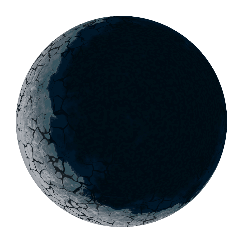
The eyeball regimes deserve their citation trail, since they are the system's most exotic-looking and best-grounded output. A tidally locked temperate world plausibly freezes on its permanent night side and thaws only near the substellar point, the "eyeball" configuration of climate modelling (Joshi, Haberle & Reynolds 1997; Pierrehumbert 2011), popularised under exactly this name (Raymond 2015). The renderer's locked ice-ocean world (open ocean at the substellar point, pack ice and floes toward the terminator, a solid cap on the far side) and its locked lava world (molten dayside pool, graduated to a dark frozen crust) are direct visual transcriptions of that literature.
2.3 Within-type positioning
Classification is not the end of the data's influence. Temperate worlds are positioned within the habitable zone by the Kopparapu polynomials evaluated for the actual host star: the planet's S_eff is normalised between the computed runaway-greenhouse and maximum-greenhouse fluxes, nudged by a logarithmic mass term, and the result interpolates every surface parameter, sea level, ice-cap extent, cloud cover, atmospheric rim colour, along a three-anchor spline from a Mars-like state through an Earth-like state to a hot, humid end state. Giants are similarly modulated: Saturn-like pallor below half a Jupiter mass, deepened banding above 1.5, a washed-out "puffy" blend for inflated radii, following the qualitative trends of the irradiated-giant literature (Sing et al. 2016). Host-star temperature selects among curated surface palettes, so that red-dwarf worlds render under redder insolation than F-star worlds, and a per-planet seed applies bounded hue jitter so that sibling planets of one type remain distinguishable.
3. The appearance layer
3.1 Noise machinery
All surfaces derive from analytic noise; there are no image textures. The foundation is classic 3D Perlin gradient noise (Perlin 1985, 2002; GLSL implementation after McEwan et al. 2012), wrapped into fractional Brownian motion families: a high-detail fBm at eight octaves (three at low level-of-detail), a ridged variant (folded and fourth-powered, for mountain chains and flow channels), a sinusoidally modulated "cloud" variant, and a 3×3×3-cell Voronoi/cellular basis (Worley 1996) for craters, ice-floe plates and lava crust. Continents, gas-giant bands and ice boundaries are all domain-warped, noise evaluated at coordinates displaced by other noise (Quílez 2002–2008; the two-stage warp on the giants follows the canonical construction), which is what moves the output from static on a sphere toward geology. The star surface runs a separate 4D simplex fBm (five octaves) so that granulation animates in time; a temperature-derived tint applies an approximate blackbody colour continuously from M-dwarf orange to O-star blue.
3.2 The regime shaders
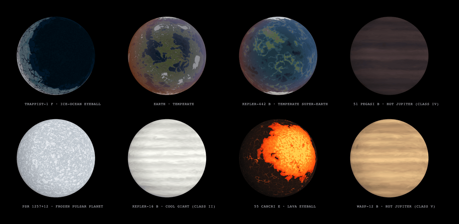
Seven fragment programs cover the sixteen types.
Gas giants
The giant program advects its noise field with a latitude-dependent Coriolis rotation (fast equator, slow poles), lays banding as a sine of warped latitude whose frequency is a per-type uniform, seeds a handful of anticyclonic storm vortices with compressed, cubic-falloff eyes, roughens band boundaries with edge turbulence, and darkens poles and storm cores. Class V giants add thermal emissive glow; ice giants swap to methane blues with faint banding, a Neptune-like dark-spot pair, and their own limb darkening.
Terrestrial worlds
The terrestrial program builds a continent function from three domain-warped fBm layers with an S-curve contrast push around a sea level set by classification; ocean colour grades through deep, mid and shallow water with a coastal shelf; land is zoned by latitude and a moisture field into wet and arid lowlands, highlands, tundra, exposed rock and snow-capped peaks; four scales of procedural bump normals (terrain gradient, ridged chains, hills, micro-detail) light the relief; polar caps grow with domain-warped, noise-jittered edges. Ocean pixels receive a specular lobe (Blinn-style, exponent 32) gated by the terminator.
Locked eyeball worlds
The locked regimes replace latitude zoning with substellar-angle zoning: the ice-ocean case keeps open water under the star, then slush, then pack ice with Voronoi crack networks (dark seawater in the cracks), then a solid cap on the night side; the lava case renders a molten pool graded through a seven-stop temperature ramp toward a dark basalt night side, with lava rivers along major Voronoi edges and residual-heat seams on the cold hemisphere.
Cloud layers
Clouds are a separate translucent sphere (radius 1.006, temperate and water worlds only) with four superposed systems, domain-warped cumulus masses, stretched cirrus wisps, ridged frontal boundaries and fine convective texture, together with an ITCZ band at the equator and Hadley-like banding at a per-type frequency; on locked worlds the entire layer reorganises into a logarithmic-spiral hurricane centred on the substellar point, with a cleared eye, feathered arms, and a convergence band at the terminator. Coverage is thresholded, so classification tunes cloudiness; edges are eroded by noise; and the layer fades out across the terminator.
Hazy, airless and frozen worlds
The remaining programs cover hazy worlds (sub-Neptunes and Venus analogues: thick domain-warped cloud tops, slow rotation) and airless or frozen rocky worlds (ridged terrain with four scales of Voronoi cratering; lava variants swap craters for flow-warped noise, emissive in the lows, and on locked hot rocks a day–night glow gradient from 8 % to 200 %).
3.3 Lighting and atmosphere
Lighting is deliberately a stylised model, not radiative transfer. The diffuse term is wrap lighting, light = clamp(((N·L)·w + w)^p, 0, 1), a long-standing real-time softening of the terminator (the half-Lambert family; Mitchell, McTaggart & Green 2006), with wrap w and power p exposed as uniforms and tuned project-wide (w = 0.65, p = 4). A fresnel-squared rim term stands in for limb ambience, scaled by an ambient uniform whose default is zero: night sides are dark. The atmosphere is a single fresnel-mixed shell whose rim colour interpolates from a twilight tone to a day tone across the terminator, masked by the same wrap function; this is an intentionally cheap approximation in place of physically based scattering (Nishita et al. 1993; Bruneton & Neyret 2008), and it is one of the paper's clearly flagged fidelity ceilings.
Determinism is total. Given one catalogue record and one seed, every octave of every noise call is reproducible; the same world renders on every machine, in the live viewer and in the baked thumbnails alike (companion paper, §3.7).
4. The speculation gradient
The system's claim rests on being able to say, for any visible feature, which kind of statement it is. We grade four tiers.
Tier 1: measured
Orbital period, semi-major axis, eccentricity, radius and/or minimum mass, stellar temperature, radius and mass, distance. These come from the catalogue with published uncertainties, which the renderer does not yet surface, a stated limitation. Visual consequences: orbital motion, relative sizes, star colour.
Tier 2: derived
Bulk density, S_eff, T_eq, habitable-zone position. Deterministic arithmetic on tier 1, inheriting its gaps: T_eq assumes zero albedo, and density inherits the mass–radius fallback where one input is missing. Visual consequences: which side of each classification threshold a planet falls.
Tier 3: theory-guided inference
The planet types themselves. That a 1.4 R⊕ planet at S_eff 0.9 is "temperate", that a ρ < 2 world is volatile-rich, that a close-in rocky planet is locked, that a 1600 K giant carries silicate clouds: each is a defensible reading of the literature (Kopparapu 2013; Fulton 2017; Zeng 2019; Barnes 2017; Sudarsky 2000, 2003), and each could be wrong for any individual planet. The observed diversity of the population, clear and cloudy hot Jupiters at the same temperature (Sing et al. 2016), guarantees a nonzero per-planet error rate that no threshold tree can remove. Visual consequences: everything categorical, ocean or lava, banded or blue.
Tier 4: fictive
Continent shapes, shoreline fractality, cloud configurations, storm placements, crack networks, palette jitter. These are hash functions. They are constrained fiction, a temperate world's fiction drawn from Earth-like morphology, a locked world's from eyeball climate states, but no pixel of them is knowledge. The system's one unbreakable rule is that tier 4 must never be adjusted per planet by hand: the moment a specific world's continents are art-directed, the pipeline's claim to be a function of the data is forfeit.
Stated as a ceiling: the renderer offers plausibility, not prediction. It is a visual hypothesis generator whose hypotheses are typed, sourced and reproducible, closer to a climate-model schematic than to a photograph, and closer to a photograph than to a table. The appropriate reading of any rendered world is a planet of this measured kind could look like this, and never this planet looks like this.
This grading also clarifies the relationship to the artist's impression. The difference is not talent (a skilled artist encodes more atmospheric science in a single matte painting than this shader knows) but auditability: here the mapping from record to image is code, versioned, uniform across four thousand systems, and gradable tier by tier. The genre-level argument is continued in the third companion paper.
5. Related work
Planetary procedural generation
The techniques are graphics-canonical: gradient noise and its fBm assemblies (Perlin 1985, 2002; Musgrave et al. 1989; Ebert et al. 2003), cellular bases (Worley 1996), GLSL noise implementations (McEwan et al. 2012), domain warping (Quílez). Whole-planet procedural systems are mature in entertainment; Space Engine renders a procedurally infinite universe seeded by real catalogues where available, and No Man's Sky (Hello Games 2016) generates worlds at galactic count. But their generators optimise variety and wonder, not fidelity to a specific record, and neither documents a per-feature epistemic grading. Scientific-visualisation systems (Eyes on Exoplanets; OpenSpace, Bock et al. 2020) conversely tend to use stock class imagery rather than per-record synthesis. The niche claimed here is narrow but real: per-record, literature-thresholded, tier-graded procedural appearance over a complete public catalogue.
Exoplanet characterisation
The classification leans on the mass–radius and demographics literature (Weiss & Marcy 2014; Rogers 2015; Fulton et al. 2017; Chen & Kipping 2017; Zeng et al. 2019), the habitable-zone formulation of Kopparapu et al. (2013) after Kasting et al. (1993), giant-atmosphere theory (Sudarsky et al. 2000, 2003; Madhusudhan 2019), locked-world climatology (Joshi et al. 1997; Pierrehumbert 2011), and the direct appearance constraints cited in §1.1. The renderer contributes nothing to that literature; it is a consumer with citations.
6. Evaluation design
Not yet run; specified for the record.
Classification audit
Sample ~100 catalogue planets stratified across the tree's branches, including all with published characterisation (TRAPPIST-1 b–h, GJ 1214 b, 55 Cnc e, HD 189733 b, the HR 8799 giants, known super-puffs); have two exoplanet researchers independently assign types from the same input vector; report agreement with the tree per branch (Cohen's κ), and, the more interesting number, the cases where the literature contradicts the tree (GJ 1214 b's flat spectrum, for example, demands cloud or haze cover that density alone would not assign; Kreidberg et al. 2014).
Can readers tell what is invented?
Show readers rendered worlds with and without a tier-graded legend ("measured / inferred / illustrative"); measure whether the legend shifts stated confidence about specific features ("does this planet have continents?" should move from majority-yes toward majority-unknown). This directly tests whether graded speculation can be communicated and not merely documented.
Determinism regression
A pixel-hash test across GPUs and drivers for a fixed record set, since the reproducibility claim ("same record, same world") is in practice bounded by floating-point and driver variance; the deviation should be measured, not assumed zero.
7. Limitations
The tree is thresholds, not posteriors
A planet at S_eff 1.05 renders Venus-like; at 1.03, temperate. Real inference would be probabilistic in the measurement uncertainties, which the catalogue provides and the classifier ignores. Rendering the modal world where the data straddle a boundary overstates confidence exactly there.
T_eq ignores albedo; the locking heuristic ignores time
Both are acknowledged coarse proxies (§2.1); both gate categorical visual outcomes.
Earth-centrism of the fictive tier
Cloud systems are Earth's (ITCZ, Hadley bands, cyclonic spirals); temperate palettes are Earth biomes hue-shifted by stellar class. The fiction is drawn from a sample of one inhabited atmosphere, and the true morphological diversity of temperate exoplanets is unknowable from it.
No radiative transfer, no spectra
Colours are palette assignments guided by the literature, not forward-modelled from atmospheres; the one planet with a measured colour (HD 189733 b) is matched by class, not computed.
Sparse records render with undiminished confidence
The interface does not yet distinguish a fully characterised planet from an m sin i-only detection, a limitation shared with the companion paper; the "what is this picture based on?" affordance is the highest-priority roadmap item this analysis motivates.
The plausibility claim is untested
Until the audit and perception studies run (§6), "plausible" is the author's judgement with citations, not a measured property.
8. Conclusion
A catalogue holds planets as vectors of numbers; readers imagine them as places. This method makes the conversion inspectable. The classification has published thresholds and sources. The appearance function has named machinery and stable seeds. Each visible choice is marked as measured, derived, theory-guided or fictive.
No shader can tell us what TRAPPIST-1 e looks like. It can show four thousand data points as worlds permitted by the evidence, with a record of every choice made along the way. Whether that helps public understanding more than the alternatives is the question for the companion survey.
Acknowledgements
The classification stands entirely on the exoplanet characterisation literature cited throughout; the shading stands on four decades of procedural graphics beginning with Perlin. Errors of reading in either direction are the author's.
References
Exoplanet characterisation and demographics
- Kasting, J. F., Whitmire, D. P., & Reynolds, R. T. (1993). Habitable Zones around Main Sequence Stars. Icarus 101, 108–128.
- Joshi, M. M., Haberle, R. M., & Reynolds, R. T. (1997). Simulations of the Atmospheres of Synchronously Rotating Terrestrial Planets Orbiting M Dwarfs. Icarus 129, 450–465.
- Sudarsky, D., Burrows, A., & Pinto, P. (2000). Albedo and Reflection Spectra of Extrasolar Giant Planets. ApJ 538, 885–903.
- Sudarsky, D., Burrows, A., & Hubeny, I. (2003). Theoretical Spectra and Atmospheres of Extrasolar Giant Planets. ApJ 588, 1121–1148.
- Knutson, H. A., et al. (2007). A map of the day–night contrast of the extrasolar planet HD 189733b. Nature 447, 183–186.
- Marois, C., et al. (2008). Direct Imaging of Multiple Planets Orbiting the Star HR 8799. Science 322, 1348–1352.
- Pierrehumbert, R. T. (2011). A Palette of Climates for Gliese 581g. ApJ Letters 726, L8.
- Majeau, C., Agol, E., & Cowan, N. B. (2012). A Two-dimensional Infrared Map of the Extrasolar Planet HD 189733b. ApJ Letters 747, L20.
- Evans, T. M., et al. (2013). The Deep Blue Color of HD 189733b: Albedo Measurements with Hubble Space Telescope/STIS. ApJ Letters 772, L16.
- Kopparapu, R. K., et al. (2013). Habitable Zones around Main-sequence Stars: New Estimates. ApJ 765, 131.
- Kreidberg, L., et al. (2014). Clouds in the atmosphere of the super-Earth exoplanet GJ 1214b. Nature 505, 69–72.
- Weiss, L. M., & Marcy, G. W. (2014). The Mass–Radius Relation for 65 Exoplanets Smaller than 4 Earth Radii. ApJ Letters 783, L6.
- Rogers, L. A. (2015). Most 1.6 Earth-radius Planets Are Not Rocky. ApJ 801, 41.
- Raymond, S. (2015). Forget "Earth-Like" — We'll First Find Aliens on Eyeball Planets. Nautilus, February 2015.
- Sing, D. K., et al. (2016). A continuum from clear to cloudy hot-Jupiter exoplanets without primordial water depletion. Nature 529, 59–62.
- Demory, B.-O., et al. (2016). A map of the large day–night temperature gradient of a super-Earth exoplanet. Nature 532, 207–209.
- Barnes, R. (2017). Tidal locking of habitable exoplanets. Celestial Mechanics and Dynamical Astronomy 129, 509–536.
- Fulton, B. J., et al. (2017). The California-Kepler Survey. III. A Gap in the Radius Distribution of Small Planets. AJ 154, 109.
- Chen, J., & Kipping, D. (2017). Probabilistic Forecasting of the Masses and Radii of Other Worlds. ApJ 834, 17.
- Madhusudhan, N. (2019). Exoplanetary Atmospheres: Key Insights, Challenges, and Prospects. ARA&A 57, 617–663.
- Zeng, L., et al. (2019). Growth model interpretation of planet size distribution. PNAS 116, 9723–9728.
- JWST Transiting Exoplanet Community Early Release Science Team (2023). Identification of carbon dioxide in an exoplanet atmosphere. Nature 614, 649–652.
Procedural graphics and real-time shading
- Perlin, K. (1985). An Image Synthesizer. SIGGRAPH '85, 287–296.
- Musgrave, F. K., Kolb, C. E., & Mace, R. S. (1989). The synthesis and rendering of eroded fractal terrains. SIGGRAPH '89, 41–50.
- Nishita, T., Sirai, T., Tadamura, K., & Nakamae, E. (1993). Display of the Earth taking into account atmospheric scattering. SIGGRAPH '93, 175–182.
- Worley, S. (1996). A cellular texture basis function. SIGGRAPH '96, 291–294.
- Perlin, K. (2002). Improving Noise. ACM Transactions on Graphics 21(3), 681–682.
- Ebert, D. S., Musgrave, F. K., Peachey, D., Perlin, K., & Worley, S. (2003). Texturing & Modeling: A Procedural Approach, 3rd ed. Morgan Kaufmann.
- Mitchell, J., McTaggart, G., & Green, C. (2006). Shading in Valve's Source Engine. SIGGRAPH 2006 Course: Advanced Real-Time Rendering.
- Bruneton, E., & Neyret, F. (2008). Precomputed Atmospheric Scattering. Computer Graphics Forum 27(4), 1079–1086.
- Quílez, I. (2002–2008). Domain warping; fBm. Articles at iquilezles.org.
- McEwan, I., Sheets, D., Richardson, M., & Gustavson, S. (2012). Efficient computational noise in GLSL. Journal of Graphics Tools 16(2), 85–94.
Systems
- Bock, A., et al. (2020). OpenSpace: A System for Astrographics. IEEE TVCG 26(1), 633–642.
- Space Engine. https://spaceengine.org (V. Romanyuk, 2010–).
- Hello Games (2016). No Man's Sky.
Appendix A: The types at a glance
| Type | Trigger (verbatim thresholds) | Visual treatment |
|---|---|---|
| Hot Jupiter V | giant, T_eq > 1400 K | silicate tans, thermal emissive |
| Hot Jupiter IV | giant, T_eq > 900 K | alkali near-black |
| Warm giant | giant, T_eq > 350 K | cloudless azure |
| Cool giant | giant, T_eq > 150 K | water-cloud white |
| Cold giant | giant, else | ammonia bands, Jupiter-like |
| Ice giant | 3.5 < R ≤ 6 R⊕ | methane blue, dark spots |
| Lava eyeball | locked, S_eff > 25, ρ ≥ 3 | dayside melt pool, basalt night |
| Lava world | S_eff > 25, ρ ≥ 3 | global magma, emissive lows |
| Hot rocky | S_eff > 1.04, dense/small | Mercury greys, cratered |
| Venus-like | rocky, S_eff > 1.04, R > 0.5 R⊕ | thick warped haze |
| Ice-ocean eyeball | locked, ρ < 2 or HZ cold edge | substellar ocean, floe rings, night cap |
| Water world | 1.75–3.5 R⊕, ρ < 2 | deep ocean, sparse islands |
| Sub-Neptune | 1.75–3.5 R⊕, ρ unknown/mid | blue-grey haze |
| Temperate | rocky, 0.35 < S_eff ≤ 1.04 | Mars↔Earth↔hot-humid lerp by HZ position |
| Frozen | rocky, S_eff ≤ 0.35 | pale ice, ridged |
| Unknown | (defined, unreachable) | n/a |
Appendix B: Sourcing notes
- The 0.27 mass–radius exponent is used here as an engineering constant in the terran regime; Chen & Kipping's (2017) fitted terran exponent is ~0.28 with stated uncertainty, and the correspondence is approximate by design.
- The tidal-locking semi-major-axis cutoffs (0.15/0.05/0.03/0.02 AU by stellar class) are a legibility heuristic, not a fit to Barnes (2017); locking is a timescale, not a boundary.
- "Eyeball planet" is a popularising term (Raymond 2015) for configurations studied more soberly as synchronously rotating climates (Joshi et al. 1997; Pierrehumbert 2011); the renderer's iconography follows the popular term knowingly.
- Wrap-lighting values (w = 0.65, p = 4) and all palette hexes are aesthetic tuning, tier 4 in the grading used here, and are recorded in version-controlled defaults rather than claimed from any source.